The Kernel Stein Discrepancy

Stein discrepancies (SDs) calculate a statistical divergence between a known density \(\mathbb{P}\) and samples from an unknown distribution \(\mathbb{Q}\). In this post, we will introduce the Stein discrepancy, in particular the Langevin Kernel Stein Discrepancy (KSD), a common form of Stein discrepancy.

We can express Stein discrepancies as [1]:

Under mild regularity conditons, the Stein discrepancy has the statistical divergence properties [2]:

and

One common form of SDs is the Langevin Kernel Stein discrepancy (KSD), which we will describe in some detail. The KSD calculates the divergence of an unnormalised density function with samples from an unknown distribution. In many applications of statistics and machine learning, the existence of a statistical quantity with these properties is very useful. In many cases, using an unnormalised density can mitigate model intractability. We also don’t require assumptions on our unknown distribution, calculating the divergence directly from the samples. Stein discrepancies have been the source of many important research directions including the evaluation of sampling techniques and testing goodness of fit.

We will first introduce the formulation of Stein disrepancies through the lens of integral probability metrics (IPMs). Afterwards, we will go into some details of the KSD.

Integral Probability Metrics (IPMs): A Quick Review

The IPM is defined as [3]:

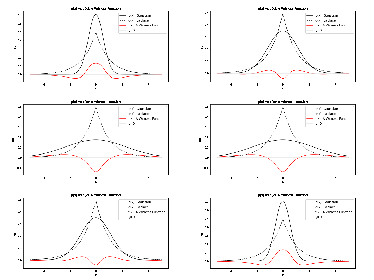
It is a comparison of two distribution under the transformation of some \(f\) in \(\mathcal{F}\). In particular, we search for \(f^*\), called the witness function, a transformation that maximimally exposes the differences of \(x \sim \mathbb{P}\) and \(y \sim \mathbb{Q}\). We can visualise possible witness functions when \(\mathbb{P}\) is Gaussian and \(\mathbb{Q}\) follows a Laplace distribution:

To find a meaningful \(f^*\), \(\mathcal{F}\) must be a large set of functions to ensure that the IPM is a metric. As you may be familiar with divergences (i.e. the Kullback Leiber Divergence), a metric is a divergence with the additional properties of symmetry and the triangle inequality. For example, if we chose \(\mathcal{F}: \{f(x) = 0\}\), then \(\mathbb{E}_{x \sim \mathbb{P}}[f(x)] - \mathbb{E}_{y \sim \mathbb{Q}}[f(y)]\) would always be zero. This would not be a metric. Another choice of \(\mathcal{F}\) is \(\mathcal{C}_b(\mathcal{X})\), the set of bounded continuous functions. This is a large enough set to ensure that the IPM is a metric, though it should be noted that the supremum in this case is not easily computable. There are many other choices of \(\mathcal{F}\) that can formulate valid IPMs.

Stein Discrepancies

The KSD quantifies the descrepancy between a known density \(\mathbb{P}\) and samples from an unknown distribution \(\mathbb{Q}\). It does this by modifying \(f\) from the IPM with a Stein Operator satisfying the Stein Identity.

The Stein Identity

Suppose we want to find an operator \(\mathcal{A_\mathbb{P}}\) such that [1]:

This is known as the Stein Identity. Any operator \(\mathcal{A}\) that satisfies the Stein identity is called a Stein operator. Using our IPM equation and applying a Stein operator to \(f\), the first term evaluates to zero using the Stein Identity and we get the Stein discrepancy [1]:

Notice that only when \(\mathbb{P} = \mathbb{Q}\), the Stein discrepancy evaluates to zero, as we expect. For the Stein discrepancy, the set \(\mathcal{F}\) is also referred to as the Stein set. Although we are trying to calculate the discrepancy between \(\mathbb{P}\) and \(\mathbb{Q}\), you may notice that the Stein discrepancy doesn’t seem to explicitly involve \(\mathbb{P}\). It is actually incorporated in our Stein operator \(\mathcal{A}\).

The Langevin Stein Operator

Understanding Stein operators that satisfy the Stein equation remains an open problem, but there have been many formulations of \(\mathcal{A}\). One is the Langevin Stein operator [4] (proof in [A1]):

where \(p(x)\) is the density of \(\mathbb{P}\). In machine learning, this is often called the Stein operator. As we expect, \(\mathbb{P}\) is still present in our Stein discrepancy, but embedded into our Stein operator. We will denote the Stein operator \(\mathcal{A_{\mathbb{P}}}\) to indicate this explicitly:

From the definition of the Langevin Stein operator, we can rewrite (derivation in [A2]):

Now that we have a concrete example of a Stein operator, let’s discuss methods of calculating \((\mathcal{A_{\mathbb{P}}}f)\) on \(\mathbb{Q}\) samples.

Langevin Stein Kernels

By choosing the Stein set \(\mathcal{F}\) as the unit-ball of a reproducing kernel Hilbert space (RKHS), we can take advantage of kernel methods to compute the Langevin Stein discrepancy.

A unique kernel is defined by a chosen RKHS, having the dot product:

where \(f\) is the set of functions restricted in the unit-ball, \(\|f\|_{\mathcal{RKHS}} \leq 1\).

Applying our Langevin Stein operator:

Deriving the corresponding Langevin Stein kernel ([A3] for full derivation):

The Langevin Stein kernel is a modification of a kernel with \(p(x)\), the density of \(\mathbb{P}\).

Numerical Convergence

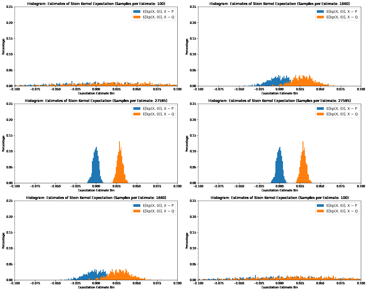
We can verify our Stein identity using the Langevin Stein Kernel:

where \(x \in \mathbb{R}^d\), by plotting the distribution of expectations of samples of \(k_{\mathbb{P}}(X, x)\). The below plot compares \(X \sim \mathbb{P}\) and \(X \sim \mathbb{Q}\), where \(\mathbb{P}\) is a Gaussian distribution and \(\mathbb{Q}\) is a Laplace distribution.

The Langevin Kernel Stein Discrepancy

We have essentially arrived at the formulation of the Langevin KSD. It is defined as [1]:

where \(k_{\mathbb{P}}\) is the Stein kernel.

An unbiased estimate [5]:

Visualising Stein Kernels

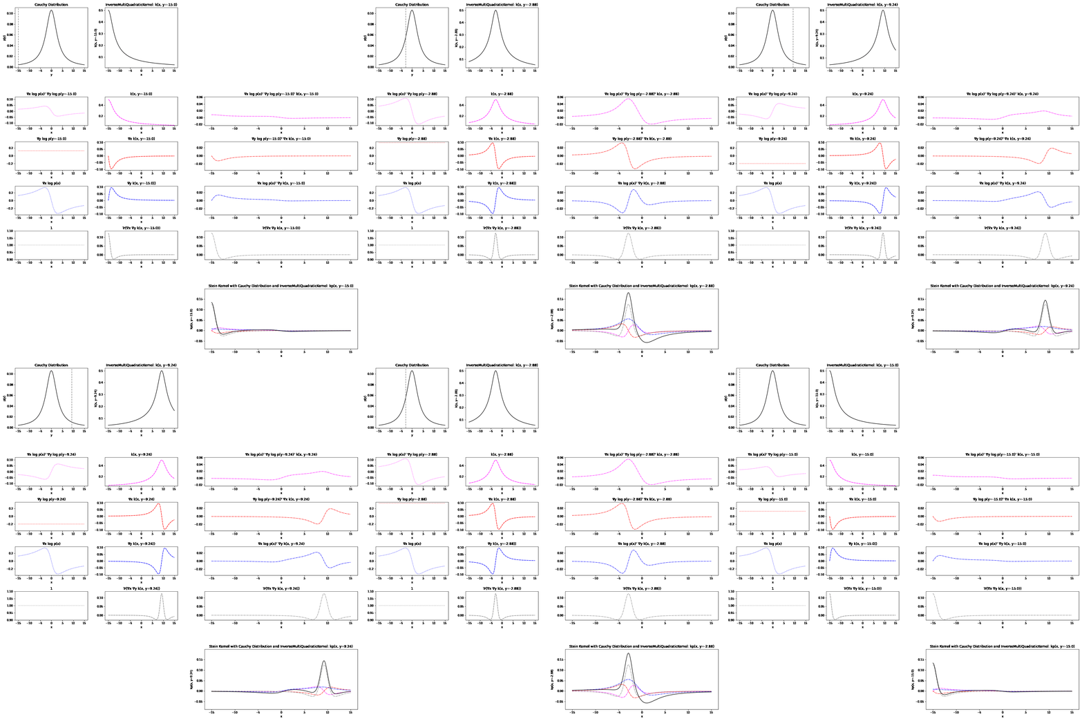
Because of their complex formulation, it can be difficult to have an intuitive understanding of Stein kernels. Visualisations may help build an understanding of what’s going on. The resulting Stein kernel can be quite complex, but we can see how they are constructed with a series of simpler components. Recall the Stein kernel:

Below, we first plot the distribution and base kernel \(k(x,y=y')\). This is followed by a breakdown of the four terms in the Stein kernel, each calculated through the product of a distribution component and a kernel component. Finally, the resulting Stein kernel is visualised as the sum of these four terms.

Here is breakdown of a Stein kernel with a Cauchy distribution and inverse multi-quadratic base kernel:

Applications of the KSD

Sampling Techniques

For many complex distributions, sampling techniques (i.e. MCMC) are important tools. Through the development of these samplers, we need to ensure that they generate data points that are genuinely representative of the underlying distribution. The KSD can help evaluate the quality of a sampler [4].

Goodness of Fit

The goodness of fit of a statistical model is fundamental to hypothesis testing in statistics. It involves quantifying the discrepancy between samples \(D = \{x_i\}_{i=1}^{N}\) and a statistical model \(\mathbb{P}_\theta\). We can compute the KSD:

which can be used for hypothesis testing [5].

Some Last Thoughts

Hopefully this was a helpful introduction to the KSD and Stein kernels! The visualisations in this blog were generated using my github repository for distribution discrepancies. Feel free to check it out!

Finally, I’d like to thank Oscar Key for helping me these past few months as I tried to wrap my head around most of these concepts. Thank you for your patience and constant feedback!

References

[1] Anastasiou, A., Barp, A., Briol, F. X., Ebner, B., Gaunt, R. E., Ghaderinezhad, F., … & Swan, Y. (2021). Stein’s Method Meets Statistics: A Review of Some Recent Developments. arXiv preprint arXiv:2105.03481.

[2] Barp, A., Briol, F. X., Duncan, A., Girolami, M., & Mackey, L. (2019). Minimum stein discrepancy estimators. Advances in Neural Information Processing Systems, 32.

[3] Müller, A. (1997). Integral probability metrics and their generating classes of functions. Advances in Applied Probability, 29(2), 429-443. Chicago

[4] Gorham, J., & Mackey, L. (2017, July). Measuring sample quality with kernels. In International Conference on Machine Learning (pp. 1292-1301). PMLR.

[5] Liu, Q., Lee, J., & Jordan, M. (2016, June). A kernelized Stein discrepancy for goodness-of-fit tests. In International conference on machine learning (pp. 276-284). PMLR. Chicago

Appendices

Appendix 1: Stein Identity Proof for the Langevin Stein Kernel

Inserting into the Stein identity, we can check that it holds:

From the definition of the expectation:

Cancelling terms:

We end up with the result:

Assuming that as \(x \rightarrow \pm\infty\) the quantities \(p(x) \rightarrow 0\) and \(f(x) \rightarrow 0\), we have satisfied the Stein Identity.

Appendix 2: Langevin Stein Operator Derivation

Unpacking the Langevin Stein operator:

Expanding:

Knowing that \(\dfrac{d}{dx} \log(f(x)) = \dfrac{f'(x)}{f(x)}\):

Defining the second term as a dot product, we have our desired formulation of the Langevin Stein operator:

Appendix 3: Langevin Stein Kernel Derivation

Starting with:

From linearity:

where \(\mathcal{A}_\mathbb{P}^x\) indicates \(\mathcal{A}_\mathbb{P}\) applied on \(x\).

Applying \(\mathcal{A}_\mathbb{P}^x\):

Note that \(\nabla_x k(x, y) = \langle \nabla_x f(x), f(y) \rangle_H\):

Applying \(\mathcal{A}_\mathbb{P}^y\):

We can rewrite \(\langle \nabla_x f(x), \nabla_y f(y)\rangle_H = \sum_i \frac{\partial k(x,y)}{\partial x_i \partial y_i} = Tr(\nabla_x \nabla_y k(x,y))\).

We arrive at the Langevin Stein Kernel: