
Gaussian Processes: A Hands On Introduction
Published:
There are many online resources for understanding Gaussian Processes. In this post, I present a more hands on way of introducing the topic that I found quite helpful and intuitive for myself.
This post will include python code from the following packages:
import math
import numpy as np
import matplotlib.pyplot as plt

np.random.seed(0)
We begin with a basic Gaussian distribution….it is called a Gaussian Process after all!
\[X \sim N(\mu, \Sigma)\]We can visualise some samples from a distribution:
k = 2
mu = np.zeros(k)
covariance = np.array(
    [
        [1.0, 0.0],
        [0.0, 1.0]
    ]
)

num_samples = int(1e4)
samples = np.random.multivariate_normal(mu, covariance, num_samples)
histogram = plt.hist2d(x=samples[:, 0], y=samples[:, 1], bins=50)
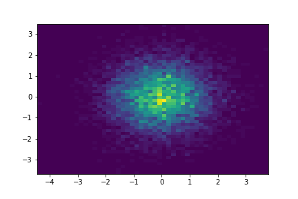
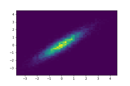
Notice how the structure of the covariance matrix can have an effect on the shape of the Gaussian:
k = 2
mu = np.zeros(k)
covariance = np.array(
    [
        [1.0, 0.9],
        [0.9, 1.0]
    ]
)

num_samples = int(1e4)
samples = np.random.multivariate_normal(mu, covariance, num_samples)
histogram = plt.hist2d(x=samples[:, 0], y=samples[:, 1], bins=50)
Identity Covariance
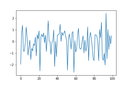
For high dimensions, we can plot a single sample with the x-axis representing each dimension of the multi-variate Gaussian. At this point, this plot looks a bit nonsensical as it’s just random noise.
k = 100
mu = np.zeros(k)
covariance = np.eye(k)

sample = np.random.multivariate_normal(mu, covariance)
fig = plt.plot(sample.transpose())
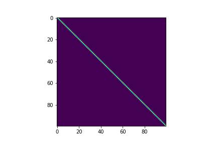
We can also visualize the covariance matrix:
fig, ax = plt.subplots()
im = ax.imshow(covariance)
RBF Kernel
We can define kernel functions, which can be interpreted as a measure of distance between two points
\[\Sigma_{i, j} = \sigma^2 \exp(-\frac{|i-j|^2}{2l^2})\]def RBF(i, j, sigma, lengthscale):
return (sigma**2)*np.exp((-(i-j)**2)/2*(lengthscale**2))
sigma = 1
lengthscale = 0.1
x = np.arange(-100, 100)
fig = plt.plot(x, [RBF(0, i, sigma, lengthscale) for i in (x)])
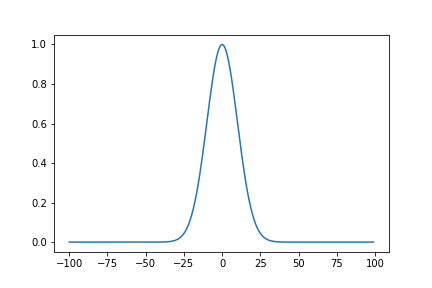
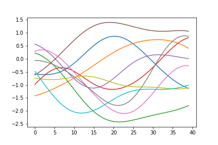
RBF Covariance
Using the kernel function to compute each element in the covariance matrix, we can generate a multi-variate Gaussian which can have desireable properties, such as smooth curves in this case. Just by changing the structure of the covariance matrix, our samples already look more interesting.
k = 40

sigma = 1
lengthscale = 0.1

mu = np.zeros(k)
covariance = np.zeros((k, k))

for i in range(covariance.shape[0]):
    for j in range(covariance.shape[1]):
        covariance[i, j] = RBF(i, j, sigma, lengthscale)
samples = np.random.multivariate_normal(mu, covariance, 10)
fig = plt.plot(samples.transpose())
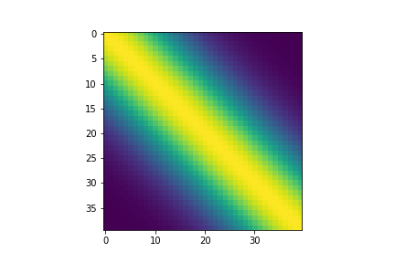
Visualizing the covariance matrix, we can see that dimensions that are “closer” to each other have higher covariance, which is the cause of the smootheness of the curves above.
fig, ax = plt.subplots()
im = ax.imshow(covariance)
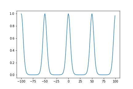
Periodic Kernel
Simiarly, we can define a periodic kernel:
\[\Sigma_{i, j} = \sigma^2 \exp(-\frac{2\sin^2(\pi|i-j|/p)}{l^2})\]def period(i, j, sigma, lengthscale, periodicity):
return (sigma**2)*np.exp(-(2*(np.sin((math.pi*np.abs(i-j))/periodicity)**2)/(lengthscale**2)))
sigma = 1
lengthscale = 0.5
periodicity = 50
x = np.arange(-100, 100)
fig = plt.plot(x, [period(0, i, sigma, lengthscale, periodicity) for i in (x)])
Periodic Covariance
This allows us to define a function space from which we can sample periodic curves
k = 40

sigma = 0.2
lengthscale = 1
periodicity = 10

mu = np.zeros(k)
covariance = np.zeros((k, k))
for i in range(covariance.shape[0]):
    for j in range(covariance.shape[1]):
        covariance[i, j] = period(i, j, sigma, lengthscale, periodicity)

samples = np.random.multivariate_normal(mu, covariance, 2)
fig = plt.plot(samples.transpose())
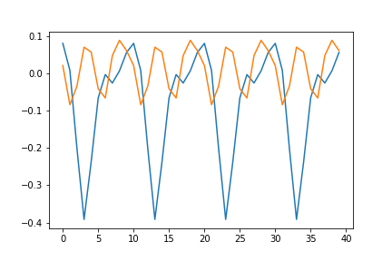
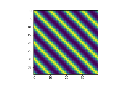
The structure of the covariance matrix also shows us how we are able to sample such curves. The periodicity is embedded into the covariance relationship
fig, ax = plt.subplots()
im = ax.imshow(covariance)
Linear Kernel
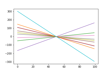
Again, we can do the same for linear functions:
\[\Sigma_{i, j} = \sigma_b^2 + \sigma^2(i-c)(j-c)\]def linear(i, j, sigma, sigma_b, offset):
return sigma_b**2+(sigma**2)*(i-offset)*(j-offset)
Periodic Covariance
k = 100

sigma = 2
sigma_b = 0.8
offset = 0

mu = np.zeros(k)
covariance = np.zeros((k, k))
for i in range(covariance.shape[0]):
    for j in range(covariance.shape[1]):
        covariance[i, j] = linear(i-int(k/2), j-int(k/2), sigma, sigma_b, offset)

num_samples = 10
samples = np.random.multivariate_normal(mu, covariance, 10)
fig = plt.plot(samples.transpose())
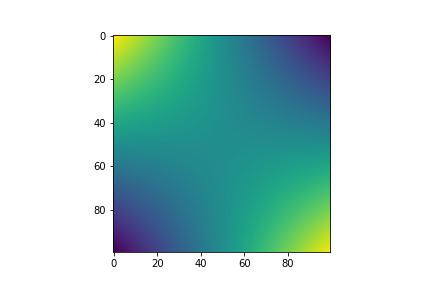
fig, ax = plt.subplots()
im = ax.imshow(covariance)
Combining Kernels
We can easily combine kernels or “function spaces” by linearly combining them when defining the covariance matrix. Here we use both the linear kernel and periodic kernel to define a function space of curves that are linear with periodic elements.
k = 100
linear_sigma = 0.1
linear_sigma_b = 0.3
linear_offset = 0

period_sigma = 1
period_lengthscale = 0.5
period_periodicity = 20

mu = np.zeros(k)
covariance = np.zeros((k, k))
for i in range(covariance.shape[0]):
    for j in range(covariance.shape[1]):
        covariance[i, j] += linear(i-int(k/2), j-int(k/2), linear_sigma, linear_sigma_b, linear_offset)

for i in range(covariance.shape[0]):
    for j in range(covariance.shape[1]):
        covariance[i, j] += period(i, j, period_sigma, period_lengthscale, period_periodicity)

samples = np.random.multivariate_normal(mu, covariance, 3)
fig = plt.plot(samples.transpose())
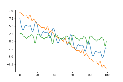
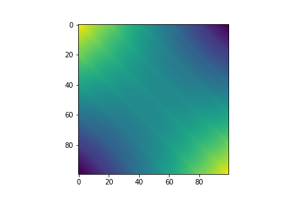
Visualizing the covariance matrix, you can see that it looks as if the linear and periodic covariance matricies from before are overlayed ontop of each other.
fig, ax = plt.subplots()
im = ax.imshow(covariance)
Conditioning
Because up until now, we’ve essentially only been working with high dimensional Gaussian distributions, we can “train” them by conditioning them on existing data. This collapses the distribution and can provide meaningful predictions for extrapolation and interpolation purposes. We can use the formula for conditioning multi-variate Gaussians:
\[X|Y \sim N(\mu_X+\Sigma_{XY}\Sigma_{YY}^{-1}(Y-\mu_Y), \Sigma_{XX}-\Sigma_{XY}\Sigma_{YY}^{-1}\Sigma_{YX})\]def condition(kernel_func, kernel_params, X, Y, X_test):
sig_xx = np.zeros((X_test.shape[0], X_test.shape[0]))
for i in range(X_test.shape[0]):
for j in range(X_test.shape[0]):
sig_xx[i, j] += kernel_func(X_test[i], X_test[j], **kernel_params)
sig_xy = np.zeros((X_test.shape[0], Y.shape[0]))
for i in range(X_test.shape[0]):
for j in range(X.shape[0]):
sig_xy[i, j] += kernel_func(X_test[i], X[j], **kernel_params)
sig_yx = np.zeros((Y.shape[0], X_test.shape[0]))
for i in range(X.shape[0]):
for j in range(X_test.shape[0]):
sig_yx[i, j] += kernel_func(X[i], X_test[j], **kernel_params)
sig_yy = np.zeros((Y.shape[0], Y.shape[0]))
for i in range(X.shape[0]):
for j in range(X.shape[0]):
sig_yy[i, j] += kernel_func(X[i], X[j], **kernel_params)
mu = np.matmul(np.matmul(sig_xy, np.linalg.inv(sig_yy)), Y)
covariance = sig_xx-np.matmul(np.matmul(sig_xy, np.linalg.inv(sig_yy)), sig_yx)
return mu.reshape(-1), covariance
kernel_func = RBF
kernel_params = {
    'sigma': 2,
    'lengthscale': 0.2,
}

X = np.array(
    [
        [0, 1, 5, 20, 21]
    ]
).transpose()
Y = np.array(
    [
        [0, 1, 0.5, 0, 1]
    ]
).transpose()

X_test = np.arange(50).reshape(-1, 1)

mu, covariance = condition(
    kernel_func,
    kernel_params,
    X,
    Y,
    X_test,
)
samples = np.random.multivariate_normal(mu, covariance, 5)
fig = plt.plot(np.repeat(X_test, 5, axis=1), samples.transpose())
fig = plt.scatter(X, Y)
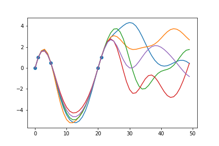
Providing a few data points to condition on, we can see that when sampling from the new posterior distribution, the curves will always pass through the given data points. This conditioning process essentially “trains” the model to take known data into account when making predictions. Hyperparameter tuning is also employed to further fine tune the model to accurately represent the behaviour of the signal and optimize the uncertainty surrounding unknown data points.